What Do “Social-Media” Features Encode? A Data Audit and Explainable Prediction of Museum Visitor Volume Across 323 Korean Museums
Abstract — A social media engagement, sentiment, and news features public dataset that describes museum visitors is cited. Data was checked before modelling. The 10 numeric columns are actual log(1+x) transformations of 10 of the columns in the attached raw data file. The headers and values (areas, counts, and a number from 0 to 365) in those columns are single letters that appear more like facility and operations attributes than social media measures. Four columns (CHN, CIP, NEWS, and COMMENTS) cannot be traced to any raw column. The column DAV is almost a copy of the target (r = 0.97), and the cross-validated R² is increased from 0.58 to 0.95. No forecasting is possible because the data are only a snapshot of 323 museums for 2023. We thus hypothesized that the number of annual visitors would be log-transformed and that there would be no leaking columns, using nested repeated 5-fold cross-validation. Random Forest (0.88 log units, 0.58 R²), XGBoost (0.90, 0.58), and ridge regression (0.92, 0.54) were not distinguishable in our experiments, and a feed-forward neural network did not perform better. The predictive signal is present in AOD and the SLV/TAV/EDA group, whereas the variables labelled as sentiment and news do not add any signal we can detect (evaluated using SHAP, permutation importance, and group ablation). The results are for prediction, and this data cannot be used to test real social media signals.
Keywords — Explainable Ai; Museum Visitor Prediction; Data Audit; Data Leakage; Shap; Cultural Heritage Analytics; Tabular Learning
I. Introduction
Museums plan their staffing, timetables and programs around the number of visitors they expect, but official counts are only confirmed later. Search data can be used to estimate gallery and museum visits [1], and a composite search index can improve tourism demand forecasting [2]. Signals from the web are also fragile. Models built on information gathered online can fail without warning [3], and information that would not be available when predictions are made can inflate accuracy for a long time without anyone noticing [4]. Explainable AI is valuable for cultural institutions because managers want to understand what influences a prediction, not only how large its error is.
A public repository [5] offers a dataset of 323 museums that is described as containing social media likes, news article views, sentiment scores and news polarity, and is intended for deep-learning prediction of museum visitors. We set out to predict how many visitors a museum would receive from those signals with sequence models and to explain the results. On examining the data we found this was not feasible, so this paper reports what the data support and what they do not. After inspection we settled on four research questions:
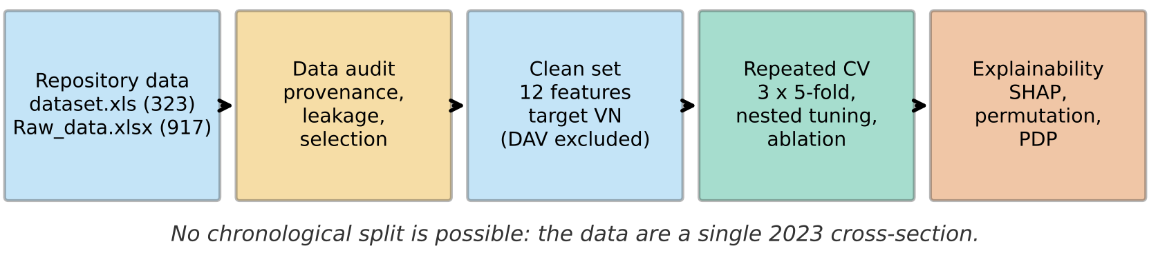
- RQ1: How accurately can log annual visitors be predicted across museums from the repository's non-leaking features (workflow in Fig. 1)?
- RQ2: Do neural networks do better than classical and tree models at this sample size?
- RQ3: Which features carry predictive signal, and do the variables labelled as sentiment and news add anything?
- RQ4: Do the repository's descriptions of its variables match where the data come from?
The paper makes four contributions: (i) an audit of the dataset's provenance and a leakage check; (ii) a leakage-free benchmark using nested, repeated cross-validation; (iii) a group ablation and explanation analysis that keeps predictive and causal readings apart; and (iv) a reproducible package of code and data.
II. Related Work
Botta et al. used Google Trends search volumes alongside monthly visits to 16 museums and galleries in the UK. Adding the search data generally improved ARIMA and neural network nowcasts compared with visit history alone, while unrelated control topics did not [1]. Li et al. found that a composite search index outperformed traditional time-series models in predicting visitor numbers to Beijing [2]. Both studies are based on real time series, which the dataset studied here does not have. Lazer et al. explain how predictors built on big data can degrade [3], and Kaufman et al. define target leakage and how to identify it [4]. We included tree ensembles because, on small tabular data, they can be competitive with or better than deep networks. We use SHAP [6] and permutation importance [7] for explanation, and we keep in mind that post-hoc explanations describe the model, not the world [8].
In the sources we reviewed, we did not find any assessment of what the columns of an open museum-visitor dataset actually contain, nor any leakage-free tabular benchmark on this data. What we offer is therefore an audit and a careful baseline, not a new forecasting model.
III. Methodology and Data Collection
Preprocessing. The features are already on a log scale, so we used them as provided. Standardization of the inputs (ridge regression and neural network) and of the target (neural network) was fitted on the training part of each fold only, so no information from the test fold leaks in. No rows were removed. Fig. 1 summarizes the workflow.
Models. Tree ensembles often perform as well as or better than deep networks on small tabular data [9]. We therefore used Random Forest [10] and XGBoost [11], and added a feed-forward neural network (FFNN) as the deep-learning candidate. A mean predictor served as a reference and ridge regression as a linear baseline. We did not use a recurrent or Transformer model because they require sequences.
Evaluation protocol. The data cannot be split chronologically, so we used 3x5-fold cross-validation [12] with seed 42. Hyperparameters were selected by an inner 3-fold cross-validation within the training folds (nested). MAE, RMSE, R² and Spearman ρ are reported on the log scale, and exp(MAE) gives a typical multiplicative error. We did not use MAPE because the target is log-transformed. Paired Wilcoxon tests on the 15 fold scores are intended only as a rough guide: the p-values are optimistic because the folds share training data, and no correction for multiple tests was applied.
Ablation and explanation. With ridge regression and XGBoost we removed one feature group at a time and also kept one group at a time (the groups follow the repository's labels; see the ablation results below). For XGBoost we used the hyperparameters selected most often in the inner search, and computed SHAP values [6] with TreeExplainer on a model fitted to all the data. Permutation importance [7] was computed on the held-out folds. Both methods describe what the model uses to predict, not what causes attendance, and we make no claim that changes in engagement or sentiment drive changes in attendance. The experimental setup, including dataset characteristics, nested cross-validation, hyperparameter tuning and model configuration, is summarized in Table I. All experiments ran on a CPU-only environment, and XGBoost was used as the explanation model.
TABLE I. Experimental configuration.
| Item | Setting |
|---|---|
| Data | 323 museums × 12 features (+ DAV excluded); target VN |
| Outer CV | 3x5-fold, seed 42 |
| Inner tuning | 3-fold, MAE; ridge α in {0.1, 1, 10, 100}; RF depth in {4, 8, None}, leaf in {1, 3, 5}, 300 trees; XGB depth in {2, 3, 4}, lr in {0.03, 0.1}, 300 trees, subsample 0.8; MLP layers in {(32), (64, 32)}, α in {0.001, 0.1} |
| Explanation model | XGBoost depth 2, lr 0.03, 300 trees |
| Environment | Python 3.13.16, scikit-learn 1.9.1, XGBoost 3.4.1, PyTorch 2.14.1+cu130 (installed, unused), CPU only, 4.8 min |
A. Dataset and Problem Formulation
We used the dataset file (18 columns, 323 rows) and the raw file (94 columns, 917 rows) from the repository [5]. They come from museum records of the Korean Culture Information Service Agency (KCISA) [13]. The repository's license text states CC BY 4.0. We credit the repository owner and KCISA; we excluded one column and made no changes to any values. The files we analyzed match the repository's: the raw file has the same SHA-256 hash and the dataset file has the same cell values. The README mentions a CSV file that is not in the repository; the data are in an .xls file.
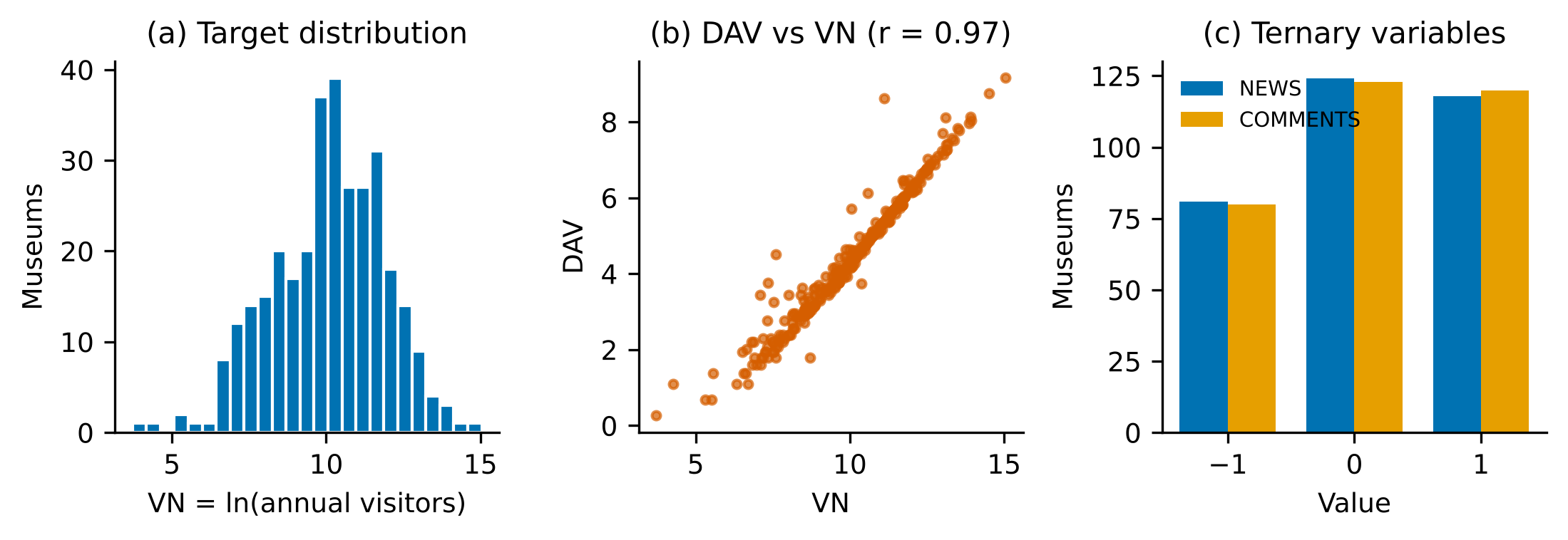
The dataset has no missing values, no duplicate rows and no duplicate IDs, and every ID appears in the raw file. There is no date or time column. The target VN equals ln(1+k) for raw column k (r = 1.0000), and k runs from 40 to 3,411,381. The README describes VN as a monthly visitor number, but values such as 3.4 million for the largest museum fit an annual total, so we interpret VN as the log of annual visitors. The raw file contains 917 museums, of which 852 have a visitor value. The 323 museums in the dataset have more visitors than the rest (mean ln visitors 10.09 against 9.43, Mann-Whitney p = 8.3e-07), and how they were selected is not documented. We flagged outliers with the IQR rule (most of them in AOD, which has 32) but did not remove any.
Each museum appears only once, so the task is to predict log annual visitors across museums (for example, to estimate volume for museums without counts). It is not a forecasting task. Chronological splits and LSTM or Transformer models do not apply here, so we did not run them and report no results for them.
B. Provenance Audit
We compared every numeric column of the dataset with every numeric column of the raw file, trying both ln(x) and ln(1+x). Ten columns match a raw column exactly (median absolute difference 0.0), while CHN, CIP, NEWS and COMMENTS match none (Table II and Fig. 2). In the raw file the matched columns are named only a to l, so we cannot state what they officially mean; Table II shows the evidence we could compute. For example, EDA has a log-log correlation of 0.96 with DSPY_AR_CN, a named area column, TPN is correlated 0.72 with the number of experience programs, and AOD never exceeds 365. These patterns fit areas, program counts and operating days much better than likes, article views or sentiment. The four unmatched columns may have been computed outside the raw file, which we cannot verify.
DAV equals ln(1+l), and l is within 2% of k/j (visitors divided by j) for 74% of the museums. Since j is at most 365, l looks like the average number of visitors per day. DAV has a correlation of 0.97 with VN, so we excluded it from all models and used the other 12 features. AOD equals ln(1+j). We kept it but flag it, because yearly totals build up over the days a museum is open, so part of its predictive power is built in. NEWS and COMMENTS take only the values -1, 0 and 1, with nearly equal counts. They are close to independent of each other (chi-square p = 0.08), and COMMENTS is not a count, as the README says it is.
TABLE II. Provenance of dataset columns. Matches are exact for ln(1+x). Raw ranges are over all raw rows; correlates use named raw columns (log-log Pearson).
| Feature | README label | Matched raw col. | Raw range | Best log-log correlate |
|---|---|---|---|---|
| SLV | avg. social likes | a | 49-3872931 | DSPY_AR_CN (0.51) |
| TAV | article views | b | 51-138156 | DSPY_AR_CN (0.72) |
| EDA | domain authority | c | 66-220695 | DSPY_AR_CN (0.96) |
| SED | sentiment embedding | d | 11-19506 | OFFM_AR_CN (0.53) |
| SA | sentiment score | e | 0-17134 | OFFM_AR_CN (0.62) |
| ND | domestic visitors | f | 17-157323 | DATA_SPCE_AR_VALUE (0.50) |
| TPN | topic centrality | i | 0-124 | FDRM_EXPRN_PROGRM_CO (0.72) |
| AOD | domain age | j | 0-365 | max = 365 (days) |
| VN (target) | monthly visitors | k | 40-3,411,381 | - |
| DAV | adjusted visitor score | l | 0.3-80,000 | about k/j (leaky) |
| CHN, CIP, NEWS, COMMENTS | see README | none | - | no raw counterpart |
IV. Results and Quantitative Comparison
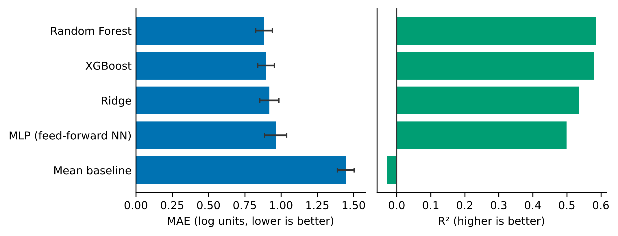
Table III and Fig. 3 give the cross-validated results for the 12 non-leaking features. Random Forest has the lowest error (MAE 0.883, or a factor of 2.42 on visitor counts), followed by XGBoost, ridge regression and the neural network. All of them beat the mean predictor (MAE 1.446). The gaps between the three best models are small compared with the spread across folds. XGBoost versus ridge gives a MAE difference of -0.022 (p = 0.21), Random Forest versus ridge -0.036 (p = 0.07), and Random Forest versus XGBoost -0.014 (p = 0.21). The neural network is worse than ridge (+0.044, p = 0.05), so for RQ2 the answer is no at this sample size. An error of about 0.9 log units means a typical prediction is off by a factor of roughly 2.4. The models rank museums fairly well (Spearman 0.76) but are not accurate enough for exact counts.
TABLE III. Cross-validated performance (log-visitor scale; mean over 15 folds; CI ignores fold overlap, so is optimistic).
| Model | MAE | RMSE | R² | Spearman | MAE ±95% CI |
|---|---|---|---|---|---|
| Random Forest | 0.883 | 1.158 | 0.585 | 0.756 | ±0.056 |
| XGBoost | 0.897 | 1.163 | 0.580 | 0.747 | ±0.056 |
| Ridge | 0.919 | 1.220 | 0.536 | 0.741 | ±0.066 |
| MLP (feed-forward NN) | 0.963 | 1.268 | 0.499 | 0.718 | ±0.077 |
| Mean baseline | 1.446 | 1.824 | -0.028 | - | ±0.058 |
When DAV is added, R² rises from 0.58 to 0.95 for XGBoost and from 0.54 to 0.95 for ridge regression, and MAE falls from 0.90 to 0.23. This jump only reflects how DAV is built from the target and says nothing about real predictive signal. Any published result that includes DAV should be read with this in mind.
A. Explainability and Ablation
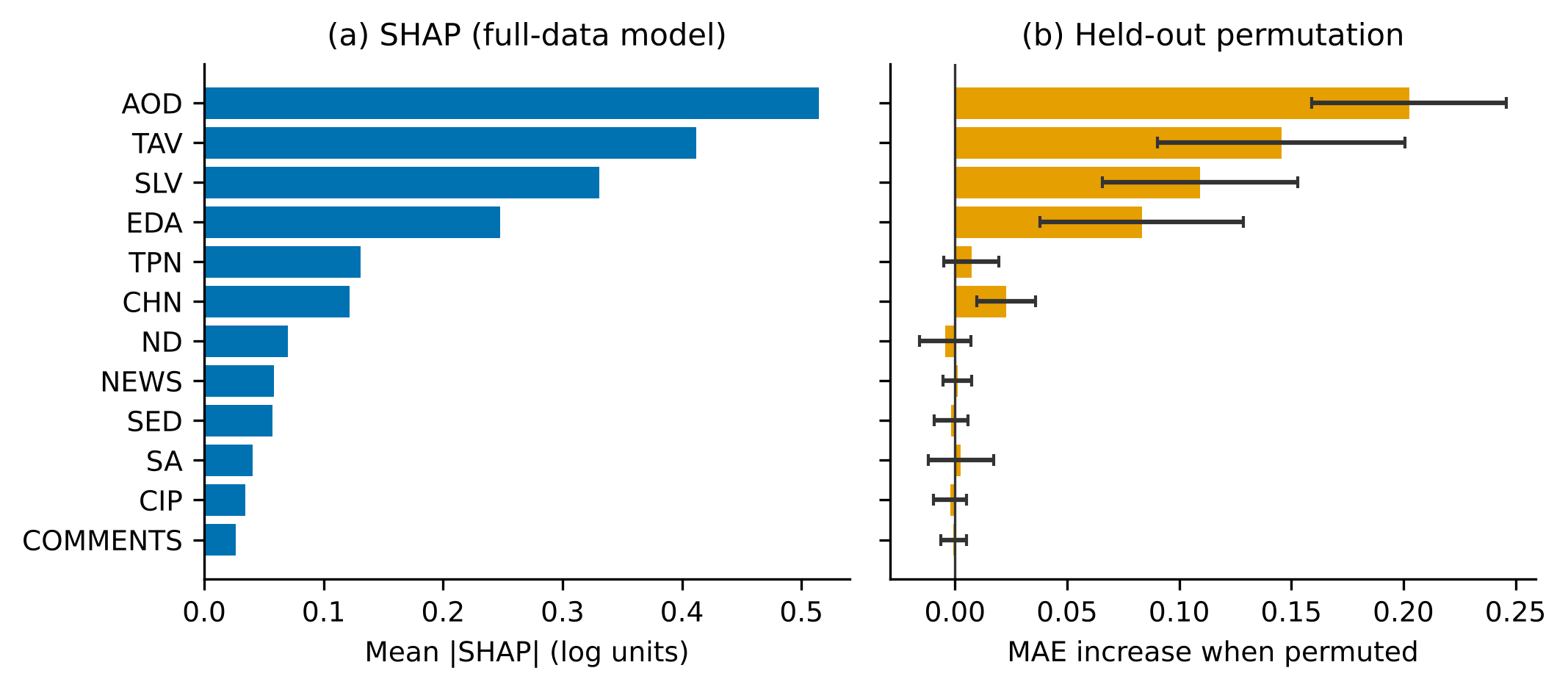
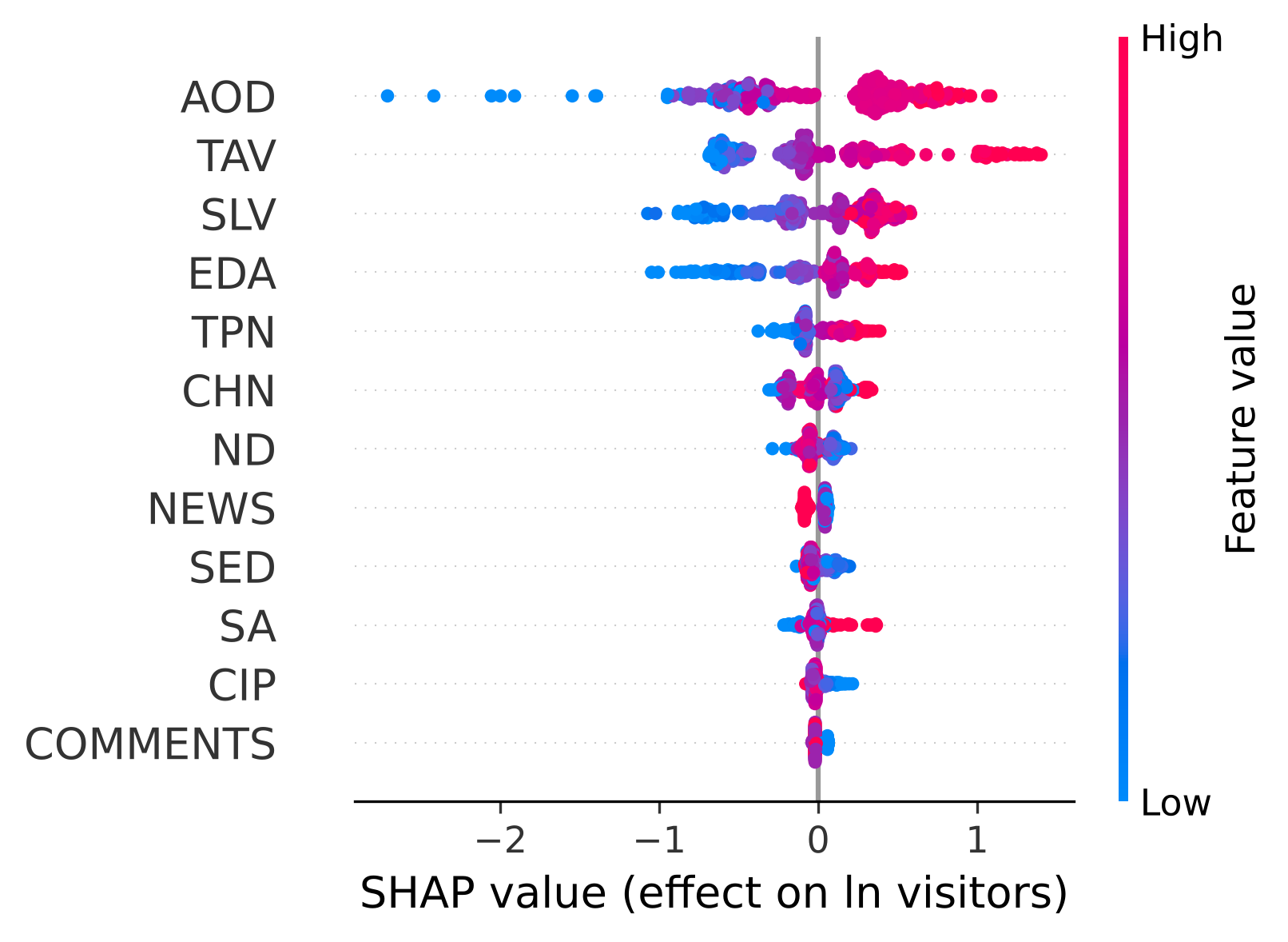
In the SHAP ranking, AOD, TAV, SLV and EDA come first (mean |SHAP| of 0.51, 0.41, 0.33 and 0.25). Permutation importance on held-out folds gives the same picture (Fig. 4). Shuffling AOD increases MAE by 0.20, TAV by 0.15, SLV by 0.11 and EDA by 0.08, while shuffling SED, SA, CIP, ND, NEWS or COMMENTS changes it by no more than 0.004, which is within noise. Fig. 5 shows the SHAP summary: museums with the fewest operating days (lowest AOD) receive strongly negative contributions, and higher values of TAV, SLV and EDA push predictions up.
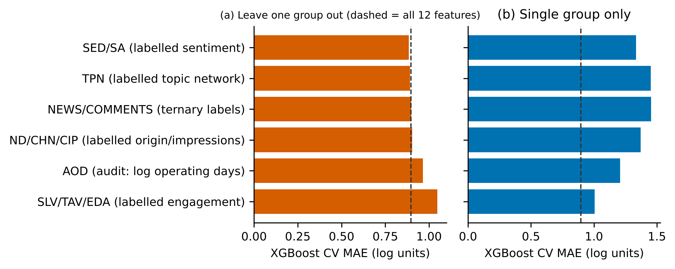
TABLE IV. Group ablation with XGBoost (full model MAE 0.897); ridge gives the same ordering (results/table_ablation.csv). p: paired Wilcoxon, descriptive.
| Feature group (repository label) | Drop: ΔMAE (XGB) | p | Only: MAE (XGB) | Only: R² (XGB) |
|---|---|---|---|---|
| SLV/TAV/EDA (labelled engagement) | +0.150 | 0.000 | 1.007 | 0.46 |
| SED/SA (labelled sentiment) | -0.012 | 0.041 | 1.335 | 0.13 |
| ND/CHN/CIP (labelled origin/impressions) | +0.007 | 0.359 | 1.370 | 0.07 |
| TPN (labelled topic network) | -0.006 | 0.454 | 1.451 | 0.00 |
| AOD (audit: log operating days) | +0.068 | 0.002 | 1.208 | 0.27 |
| NEWS/COMMENTS (ternary labels) | +0.002 | 0.847 | 1.455 | -0.04 |
Dropping SLV/TAV/EDA raises MAE by 0.150, and dropping AOD raises it by 0.068 (Table IV and Fig. 6). Dropping any other group changes MAE by at most 0.012, and the direction differs between the two learners. NEWS and COMMENTS on their own give an R² of about -0.04, which is no better than predicting the mean. We could not run the ablation planned in the original brief (attendance history only versus history plus social media), because the data contain no attendance history. For RQ3, then, the signal sits in AOD and in SLV/TAV/EDA, and the sentiment and news variables carry none that we can detect.
B. Discussion and Practical Implications
The main message for museum managers is one of caution. First, in this dataset the number of annual visitors is predicted by the size and operating features of a museum rather than by its sentiment labels, even though several of these columns are labeled as social media measures. Second, when a column is said to measure social media, its source should be checked before it is used in a dashboard or forecast. Third, judging whether social media or news sentiment really helps requires visitor counts over time and signals that line up with them, as in [1] and [2]. Fourth, the explanations here describe associations. AOD matters partly because yearly totals build up over the days a museum is open, and large museums differ from small ones in many ways we cannot see. These points answer RQ4: for at least ten columns the repository's descriptions do not match the raw data, and for four columns there is no traceable source.
C. Limitations and Threats to Validity
The data cover one year and 323 museums, and the rule used to select them is not documented. The selected museums are larger on average, so our results may not carry over to small museums. Because the raw columns are labeled only with letters, we had to infer what they represent from their values. The four columns we could not trace (CHN, CIP, NEWS and COMMENTS) may have been built outside the raw file, and we could not check this. Our random folds are not fully independent, since museums that belong to the same institution or site are related. The hyperparameter grids are small, and the paired tests and confidence intervals are optimistic because the folds overlap. The SHAP values come from a model fitted to all the data. None of the results are causal. Finally, our literature search was not systematic, and we could not open one recent museum-forecasting paper that may use this dataset, so it is not cited.
V. Conclusion and Future Work
The dataset allows a cross-sectional analysis but not a time-series analysis. Once the leaking column is removed, our models account for about 58% of the variation in log annual visitors. A simple ridge regression does almost as well as the tree models, and the variables named sentiment and news add nothing we can detect. In future work we would request documentation from the dataset authors. We would then gather true monthly attendance together with search, social media and news signals over time, and only then evaluate sequence models with rolling-origin evaluation.
VI. Acknowledgments
The data were collected by KCISA and shared by Jae Ho Lee [5] under CC BY 4.0 [13]. We excluded the column DAV and made no other changes to the values.
VII. Data Availability Statement
The data we analyzed come from the public GitHub repository "museum-visitor-deep-learning-data" (https://github.com/JaeHo0918/museum-visitor-deep-learning-data), which is released under CC BY 4.0 [5] and is based on KCISA museum records [13]. We did not change those files. The cleaned version used in this paper was produced by us from the two original files with the script data_preprocessing.py. It keeps all 323 museums and all original values, renames the column DAV as DAV_EXCLUDED_leaky so that it is not used as a predictor, and adds two helper columns (the raw visitor count and an outlier flag). The cleaned dataset (museum_clean.csv), the unchanged original files, the data dictionary, the audit tables, the saved predictions and results, and all code are placed in our own GitHub repository: https://github.com/Rana64/A-Data-Audit-and-Explainable-Prediction-of-Museum-Visitor-Volume-Across-323-Korean-Museums.git. Running run_experiments.py in that repository recreates every table and figure in this paper. The dataset authors have not documented what raw columns a-l contain or where CHN, CIP, NEWS and COMMENTS come from, so we could not verify these.